I have found curve-fitting in IDL to be somewhat of a frustrating process. There are a number of hoops you have to jump through that just make data analysis a pain. Furthermore, the IDL supplied curve fitting routine, called CURVEFIT, is not as robust as I would like. I have found that I can crash the entire IDL session with some fairly simple data and models. I have translated MINPACK-1, a very nice curve fitting package into IDL. The fitting programs are called MPFIT, MPFITFUN, and MPFITEXPR (and can be downloaded here). Here I present a short tutorial on how to use MPFITFUN and MPFITEXPR.

MPFITEXPR is generally the easiest to use interactively at the command line, while MPFITFUN is most commonly used in programs.

Collecting your data

The first step in any analysis process is to collect your data. You are in charge of that, since only you know the specific details of how your experiment is run. In general, you will have three sets of numbers:

• The "X" values - these are the independent variables of the experiment.
• The "Y" values - these are the "measured" dependent variables.
• The "Error" values - this is typically the 1-sigma uncertainty in your measurement.

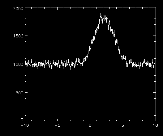
Of course you will have your own data, but I will provide some sample data (6 kb), in the form of an IDL "SAVE" file. It contains three variables, which you can imagine might represent the rate measured by a detector: t, r, and rerr, corresponding to a time, rate, and error in the rate. The error is simply the Poisson statistical error. My example below will use these variables.

Here is a plot of the data with errors:

What to do if you don't have error bars

A proper experimenter should always assign error bars to their data. After all, a data point with larger errors should be weighted less in the fit, compared to a point with small error bars. However, I can foresee that under circumstances which only you can judge, the error bars may not be relevant. In that case, you may set the "Error" term to unity and proceed with the fit. Be aware that your data may not be properly weighted, and the error estimates produced by MPFITFUN/EXPR will not be correct. Bevington (Ch. 6.4) has an approach that allows you to assign error bars once you know the best-fit sum-of-squares. This number is returned through the BESTNORM keyword.

Choosing a Model

By fitting a curve to your data, you are assuming that a particular model best represents the data. This again is up to you because of course, only you can assign an interpretation to your own data. Interpretations aside however, we can try to see how well a particular model fits by, well, just fitting it!

In this example, it is pretty clear that there is a fairly constant level of about 1000, with a "hump" near 2.5. I speculate that a constant plus Gaussian will fit that curve quite nicely. [ I in fact generated the data using that model. ]

How do you construct a model that IDL will understand? When you use MPFITEXPR, you only need to supply an IDL expression which computes the model. Here's how I would do the constant plus Gaussian model:

IDL> expr = 'P[0] + GAUSS1(X, P[1:3])'

The variable expr now contains an IDL expression which takes a constant value "P[0]" and adds a Gaussian "GAUSS1(X, P[1:3])". The GAUSS1 function is a one dimensional Gaussian curve, whose source code can be downloaded.

There are a few important things to notice here. First, the name of the independent variable is always "X", no matter what it is called in your session. When MPFITEXPR executes your expression, it substitutes the correct independent variable for "X" in the expression. Second, all of the parameters are stored in a single array variable called "P". Again, you are free to name the parameter array anything you like in your own session, but in the expression it must appear as "P".

When you use MPFITFUN instead, you need to construct an IDL function which does the same thing as the expression above. You should deposit the following function definition into a text file called mygauss.pro:

FUNCTION MYGAUSS, X, P
  RETURN, P[0] + GAUSS1(X, P[1:3])
END

and compile with:

IDL> .comp mygauss

You will need to decide for yourself how to arrange your parameter values. In my example, I decided that parameter 0, the first parameter, would be the constant value, while parameters 1 through 3 would be the parameters of the Gaussian (the three parameters to GAUSS1 are, in order: mean, sigma, and area under curve). If two parts of the expression require the same parameter value, then just type it in that way! This is a very elegant way to share parameter values between several different model components.

Choosing Starting Values

You need to at least give MPFITFUN/EXPR a starting point in the parameter space. A rough guess is fine for most problems. I can enter my guess into the IDL session like this:

IDL> start = [950.D, 2.5, 1., 1000.]

Those four numbers mean that the constant value will start at 950, and the Gaussian will start with a mean of 2.5, a sigma of 1, and an area of 1000. Since the data is double precision, I force the starting values to be double as well (or else MPFIT will complain). It is the fitting program's job to iterate until it finds the best solution it can.

Choosing the starting values can be somewhat of an art. For some particularly nasty problems with deep local minima, the proper choice of the starting parameters may mean the difference between converging to the global minimum or a local one. Again, only you can make this judgment.

Fitting the Curve

Finally we can fit the curve using MPFITEXPR or MPFITFUN on the command line:

IDL> result = MPFITEXPR(expr,     t, r, rerr, start) or
IDL> result = MPFITFUN('MYGAUSS', t, r, rerr, start)

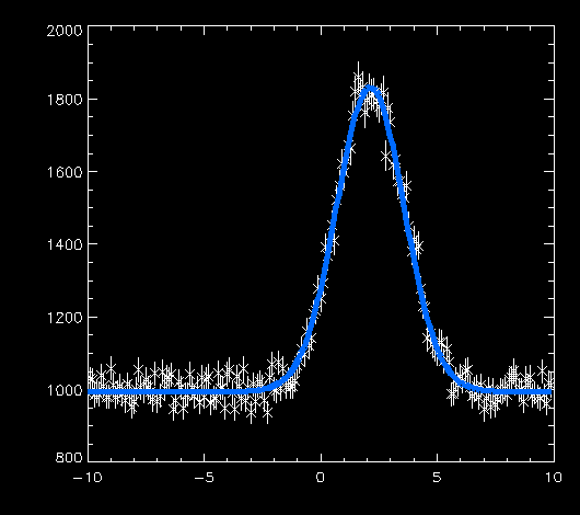
This will tell MPFITEXPR or MPFITFUN to fit the time/rate/error data using the model specified in the expression expr and starting at start. The routine will print diagnostic messages showing its progress, and finally it should converge to an answer. When it is done, we can print the results:

IDL> print, result
  997.61864 2.1550703 1.4488421 3040.2411

which means that the best-fit constant level is 997, the mean of the "hump" is 2.15 with a width of 1.45, and the area under the hump is 3040. That's all there is too it!

Verifying the Fit

As a final step in the fitting process, we can make a plot of the data and overlay a fitted model:

IDL> ploterr, t, r, rerr
IDL> oplot, t, result(0)+gauss1(t, result(1:3)), color=50, thick=5

In the oplot command above, I substituted the proper names for the independent variable and the parameter array. The color and thick keywords make the fitted curve stand out a little better. The results are excellent:

Advanced Topics: Constraining Parameters

Fixing Parameters

Now let's say that I have learned that the constant level should be fixed at 1000 exactly. I need to redo the analysis, and "freeze" the constant to 1000. One way to do that would be to rewrite the expression, and hard-code the value of 1000. Another more natural way to achieve the same thing is to "fix" the value to 1000 within the logic of MPFIT itself. All of the MPFIT functions understand a special keyword called PARINFO which allows you to do this.

You pass an array of structures through the PARINFO keyword, one structure for each parameter. The structure describes which parameters should be fixed, and also whether any constraints should be imposed on the parameter (such as lower or upper bounds). The structures must have a few required fields. You can do this by replicating a single one like this:

IDL> pi = replicate({fixed:0, limited:[0,0], limits:[0.D,0.D]},4)

A total of four structures are made because there are four parameters. Once we have the blank template, then we can fill in any values we desire. For example, we want to fix the first parameter, the constant:

IDL> pi(0).fixed = 1
IDL> start(0) = 1000

I have reset the starting value to 1000 (the desired value), and "fixed" that parameter by setting it to one. If fixed is zero for a particular parameter, then it is allowed to vary. Now we run the fit again, but pass pi to the fitter using the PARINFO keyword:

IDL> result = MPFITEXPR(expr,     t, r, rerr, start, PARINFO=pi)
IDL> result = MPFITFUN('MYGAUSS', t, r, rerr, start, PARINFO=pi)

You interpret the results the same way as before. It should be clear that the first parameter remained fixed at 1000 rather than varying to 997.

Specifying Constraining Bounds

All of the fitting procedures here also allow you to impose lower and upper bounding constraints on any combination of the parameters you choose. This might be important, say, if you need to require a certain parameter to be positive, or be constrained between two fixed values. The technique again uses the PARINFO keyword. You see above that in addition to the fixed entry, there are some others, including limited and limits. They work in a similar fashion to fixed.

For example, let us say we know a priori that the Gaussian mean must be above a value of 2.3. I need to fill that information into the PARINFO structure like this:

IDL> pi(1).limited(0) = 1
IDL> pi(1).limits(0) = 2.3

Here, for parameter number 1, I have set limited(0) equal to 1. The limited entry has two values corresponding to the lower and upper boundaries, respectively. If limited(0) is set to 1, then the lower boundary is activated. The boundary itself is found in limits(0), where I entered the value of 2.3. The same logic applies to the upper limits (which for each parameter are specified in limited(1) and limits(1)). You can have any combination of lower and upper limits for each parameter. Just make sure that you set both the limited and limits entries: one enables the bound, and the other gives the actual boundary value.

Concluding Remarks

Well, those are the basics of fitting with MPFITEXPR and MPFITFUN. You will need some practice before you can feel comfortable, which is true for anything new. I have documented the usage of each function in the header of the program file. If you need to find more information about the techniques I used above, you may find it there. If you are concerned about error analysis, then you will want to check the parameters called PERROR, COVAR and BESTNORM, which return the 1-sigma parameter errors, covariance matrix and the best-fit chi squared value.

References

Bevington, P. R. and Robinson, D. K. 1992, Data Reduction and Error Analysis for the Physical Sciences, 2nd Ed., McGraw-Hill, Inc.

Files